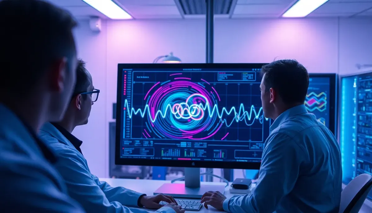
Real-time monitoring system tracks rapid fluctuations of qubits.
- Türker Şentürk
- Technology
- 20 Feb, 2026
- 11 min read
Real‑Time Qubit Watchdogs: How a Copenhagen Team Turned a Millisecond Mystery into a Quantum Advantage
When I first walked into the Niels Bohr Institute (NBI) for a “quick chat” with a postdoc, I expected the usual tour of cryogenic rigs, a few chalk‑filled whiteboards, and the occasional joke about Schrödinger’s cat being on a coffee break. What I got instead was a glimpse of a tiny, humming FPGA board that, according to the researchers, could see a qubit’s mood swing in the time it takes you to blink.
If you’ve ever tried to drive a sports car on a road that’s constantly sprouting potholes, you’ll understand why that matters. The car (your quantum processor) might be built for blistering speed, but if the surface changes faster than you can react, you’ll end up with a lot of wasted torque—and in the quantum world, that waste shows up as lost information.
The breakthrough announced on 20 February 2026 by the NBI team—led by postdoctoral researcher Dr. Fabrizio Berritta—doesn’t just give us a faster speedometer; it hands us a real‑time dashboard that can spot a qubit’s “bad day” the instant it happens. In plain English: they built a system that tracks fluctuations in a qubit’s relaxation rate about a hundred times faster than the best prior techniques.
Below, I unpack why that matters, how they pulled it off with a mix of off‑the‑shelf hardware and clever Bayesian math, and what this could mean for the race to scalable quantum computers.
Why Qubits Are So Fidgety
A qubit is the quantum analogue of the classical bit, but instead of being a simple 0 or 1, it can sit in a superposition of both. That superposition is fragile: any interaction with the environment—thermal photons, stray magnetic fields, microscopic material defects—can cause the qubit to “relax” (lose energy) or “dephase” (lose phase coherence).
In superconducting qubits, the dominant loss channel is energy relaxation, quantified by the T₁ time. A long T₁ is good; a short one means the qubit dumps its quantum information quickly. Historically, we measured T₁ by repeatedly preparing a qubit, waiting a set delay, and reading it out—a process that can take seconds to minutes per data point.
That approach gave us an average T₁—a useful number, but one that hides a lot of drama. Imagine trying to gauge a runner’s speed by only looking at their average lap time over an hour, while in reality they sprint, jog, and sometimes trip every few seconds. The average tells you nothing about those sudden drops in performance.
Enter the “fluctuation” problem: microscopic two‑level systems (TLS)—tiny defects in the materials that make up the qubit—can hop around, changing the local electromagnetic environment. When a TLS flips, the qubit’s T₁ can swing from a comfortable 100 µs to a miserable 20 µs in milliseconds. Until now, we simply didn’t have a way to see those swings as they happened.
The Old Way of Watching Qubits (and Why It Was Like Watching Paint Dry)
Standard quantum‑characterization tools rely on a classical computer that sits in the control room, collects raw measurement data from the cryostat, and then runs heavy post‑processing. Even the fastest commercial quantum‑control platforms needed tens of milliseconds to seconds to compute a new estimate of the relaxation rate after each measurement.
That lag meant the controller was always playing catch‑up, reacting to a qubit’s state after the environment had already moved on. It’s a bit like a weather app that only updates after the storm has passed.
Because of this latency, researchers were forced to average over many repetitions, effectively smoothing out the spikes. The result: a clean‑looking T₁ curve that, in reality, was a series of jagged peaks and valleys hidden beneath a statistical blanket.
The Copenhagen Hack: FPGA Meets Bayesian Brain
The NBI team’s answer was elegant in its simplicity: use a fast, programmable classical processor—an FPGA (Field‑Programmable Gate Array)—to do the heavy lifting right at the hardware level.
What’s an FPGA, and why does it matter?
Think of an FPGA as a Lego set of logic gates that you can rewire on the fly. Unlike a general‑purpose CPU, an FPGA can execute a specific algorithm in parallel, with deterministic timing down to the nanosecond. In the quantum lab, that translates to no bottleneck from data‑transfer overhead.
The researchers chose the OPX1000 from Quantum Machines, a commercial controller that can be programmed in a Python‑like language (called Quantum Orchestration Language). This lowered the barrier for other labs to adopt the technique—no need to write VHDL from scratch.
Bayesian Updating on the Fly
The core of the method is a real‑time Bayesian estimator. After each single‑shot measurement of the qubit (i.e., after the qubit is prepared, allowed to evolve for a short time, and then read out), the FPGA updates a probability distribution for the relaxation rate, Γ = 1/T₁.
Mathematically, if we denote the prior distribution as P(Γ|dataₙ₋₁) and the likelihood of the new measurement as L(dataₙ|Γ), Bayes’ rule gives:
[ P(Γ|dataₙ) \propto L(dataₙ|Γ) \times P(Γ|dataₙ₋₁) ]
The clever part is that the FPGA can compute the likelihood for a pre‑computed grid of Γ values in a few clock cycles, then perform the multiplication and renormalization instantly. The result is a posterior distribution that reflects the most up‑to‑date belief about the qubit’s relaxation rate.
Because the update happens after every single measurement, the controller’s estimate tracks the qubit’s instantaneous behavior, not a lagged average. In practice, the team reported updates every 10 µs, matching the timescale of the observed fluctuations.
Speed Gains in Numbers
| Metric | Traditional Method | FPGA‑Based Real‑Time |
|---|---|---|
| Update latency | 10–100 ms (often >1 s) | ≈10 µs |
| Number of measurements per estimate | 10⁴–10⁵ | 10–100 |
| Effective bandwidth | ~10 Hz | ~10 kHz |
| Speed‑up factor | 1× | ≈100× |
That jump is not just a technical curiosity; it reshapes how we think about calibrating a quantum processor.
Seeing the Unseen: What the Data Actually Look Like
When the team ran the new system on a standard transmon qubit (the workhorse of most superconducting platforms), the T₁ trace turned into a strobe‑light movie of relaxation rates.
- Stable periods: For a few hundred microseconds, T₁ hovered around 120 µs.
- Sudden drops: In ~5 % of the time, a TLS flipped, and T₁ plunged to 30 µs for just 20–30 µs before bouncing back.
- Burst clusters: Occasionally, multiple TLS events overlapped, creating a cascade of short‑lived “bad” qubits.
The researchers could now catalog each dip, measure its duration, and even correlate it with external variables like temperature drifts or microwave drive power. In other words, the qubit’s “mood swings” became a data set you could actually analyze, rather than a vague feeling you sensed but couldn’t quantify.
Why Real‑Time Tracking Is a Game‑Changer
1. Dynamic Error Mitigation
Error‑correcting codes (like the surface code) assume a relatively stable error rate across the qubits in a chip. If a single qubit’s error probability spikes for a few microseconds, the decoder can misinterpret that as a logical error, potentially corrupting the entire computation.
With real‑time T₁ monitoring, a control system could temporarily retire a misbehaving qubit—routing logical operations around it—in the middle of a run. Think of it as a GPS that reroutes traffic the moment an accident occurs, instead of waiting for the next daily update.
2. Accelerated Calibration
Current calibration protocols can take hours for a 50‑qubit processor, because each qubit’s parameters must be measured repeatedly. The new method can gather sufficient statistics in seconds, slashing downtime and allowing more frequent recalibration cycles.
3. Material Science Feedback Loop
Since the technique can pinpoint when and how often a TLS flips, materials scientists gain a real‑time probe of defect dynamics. That feedback could guide the next generation of thin‑film deposition recipes, substrate treatments, or even the design of qubit geometries that are less sensitive to particular defect families.
The Human Side: A Lab That Embraces “Fast‑Fail”
I asked Dr. Berritta what the most surprising thing they learned was. He laughed, “We expected the ‘good’ qubits to stay good for at least a few seconds. Turns out they can become ‘bad’ in a few hundred nanoseconds—faster than our eyes can even follow.”
That moment of surprise is a reminder that quantum hardware is still a wild frontier. The team’s willingness to experiment with commercial hardware, rather than building a custom ASIC from scratch, reflects a broader trend: pragmatic engineering over ivory‑tower perfection.
Morten Kjærgaard, the group’s associate professor, added, “Our collaboration with Quantum Machines was key. The OPX1000 gave us a ‘sandbox’ where we could iterate the Bayesian algorithm in weeks, not months.”
It’s a refreshing contrast to the usual narrative of “secret‑lab breakthroughs” that never see the light of day. Here, the tools are openly available, and the software is written in a language most quantum physicists already know. That openness could democratize high‑speed qubit monitoring across the global research community.
Limitations and Open Questions
No breakthrough is without its caveats, and this one is no exception.
-
Scope of Applicability – The current demonstration focused on a single transmon qubit. Scaling the method to a multi‑qubit processor will require multiplexed readout and parallel Bayesian updates, which could stress the FPGA’s resources.
-
Root‑Cause Ambiguity – While the system can detect a fluctuation, it doesn’t explain why a particular TLS flipped. Is it phonon‑induced, magnetic, or a charge trap? Further experiments (e.g., temperature sweeps, strain tuning) are needed.
-
Latency vs. Bandwidth Trade‑off – The FPGA updates every 10 µs, but the measurement itself still takes a finite time (typically a few microseconds). For ultra‑fast fluctuations (<1 µs), the method may still lag.
-
Integration with Error‑Correction – Real‑time monitoring is only useful if the quantum control stack can act on the information fast enough. That means integrating the FPGA’s output into the pulse‑sequencing layer and the decoder—a non‑trivial software engineering challenge.
These are not show‑stoppers, but they outline a roadmap for the next few years: multi‑qubit implementations, deeper defect spectroscopy, and tighter coupling between hardware monitors and software error‑mitigation layers.
Putting It All Together: A Glimpse of the Future
Imagine a quantum computer that runs a chemistry simulation, and halfway through the algorithm a stray TLS flips, briefly degrading one qubit’s T₁. In today’s world, that dip would be invisible until after the run, possibly corrupting the result.
With the Copenhagen system, the control hardware would flag the affected qubit in real time, either:
- Temporarily re‑encode the logical qubit onto a different physical qubit, or
- Inject a fast dynamical decoupling pulse to mitigate the loss, then resume the algorithm.
In practice, that could raise the effective logical error rate by an order of magnitude—bringing us a step closer to the error thresholds needed for fault‑tolerant quantum computing (≈1 % for surface‑code implementations).
Beyond computation, the same technique could be repurposed for quantum sensing. Superconducting qubits are already being explored as ultra‑sensitive detectors of microwave photons and dark matter candidates. Real‑time monitoring would let a sensor reject spurious background events on the fly, sharpening its signal‑to‑noise ratio.
My Takeaway (and a Little Advice for the Rest of Us)
If you’ve been following the quantum race, you’ve probably heard the mantra: “hardware, software, error correction—repeat.” The Copenhagen breakthrough reminds us that hardware and software are not separate silos; they can be co‑designed to extract more information from the same physical system.
The lesson for any tech journalist (or engineer) is simple: don’t overlook the “fast” layer. In a field where we’re used to measuring things in minutes or hours, a hundred‑fold speedup can flip a research program on its head.
For readers who are tinkering with their own quantum setups, the take‑home is encouraging: you don’t need a custom ASIC to get real‑time insight. A commercially available FPGA board, a few lines of Python‑ish code, and a Bayesian mindset can give you a window into the quantum world that was previously fogged over.
And for the broader audience—whether you’re a software developer, a hardware hobbyist, or just a curious mind—this story underscores a timeless truth: the best breakthroughs often happen when you marry a cheap, off‑the‑shelf component with a clever algorithm.
So next time you stare at a blinking LED on a lab bench, ask yourself: What if I could make that LED talk back to me, instantly, about what it just saw? In the quantum realm, that question just turned into a reality.
Sources
- Berritta, F. et al. “Real‑Time Adaptive Tracking of Fluctuating Relaxation Rates in Superconducting Qubits.” Physical Review X 16 (1), 2026. DOI: 10.1103/gk1b-stl3.
- University of Copenhagen. “Quantum computer breakthrough tracks qubit fluctuations in real time.” ScienceDaily, 20 February 2026. https://www.sciencedaily.com/releases/2026/02/260219040756.htm
- Quantum Machines. “OPX1000 Quantum Orchestration Platform – Technical Overview.” https://quantummachines.co/products/opx1000
- Niels Bohr Institute. “How to improve the performance of qubits – super‑fast fluctuation detection achieved at NBI.” https://nbi.ku.dk/english/news/news26/how-to-improve-the-performance-of-qubits-super-fast-fluctuation-detection-achieved-at-nbi/
Share :
Stay Ahead in Tech
Join thousands of developers and tech enthusiasts. Get our top stories delivered safely to your inbox every week.
No spam. Unsubscribe at any time.